Formula Explanation: Explain, Debug, Improve, Convert, Optimize & Document

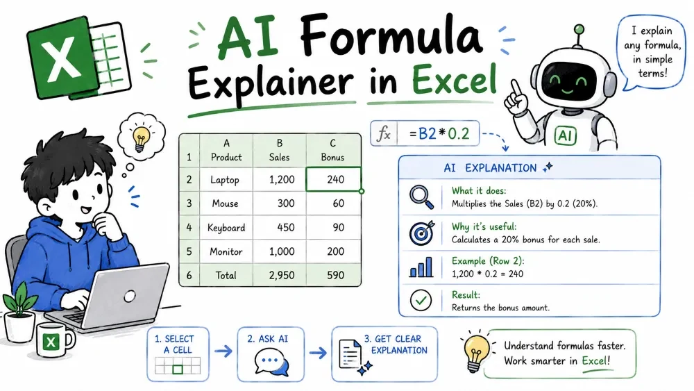
A formula does its work without ever telling you how. The six skills in this chapter change that: you take any formula you find — from a teammate, a template, or an old sheet of your own — and explain what it does, fix it when it breaks, and leave it clearer, faster, and documented than you found it. You can do all six by hand in Excel, and every one of them is also a request you can hand to AI with a short prompt.

Table of Contents

• Explain an Existing Formula
• Debug Formula Errors
• Improve a Formula
• Convert a Formula
• Optimize a Formula
• Document a Formula

Explain an Existing Formula

Explaining a formula means reading it apart so you know what it does and why — not just what number it returns. This is the skill everything else builds on. You cannot debug, improve, or document a formula you cannot read.

How to read one: read from the outside in. The function name tells you the job; the arguments inside the parentheses are its inputs. Start with the outermost function, then work into whatever sits inside its arguments.

Excel gives you tools that do the visual work:

• F2 — edit the cell; the references in the formula turn color-coded and the spreadsheet highlights the exact ranges they point to.
• Evaluate Formula (Formulas → Evaluate Formula) — steps through the calculation one piece at a time and shows you the value of each part as it runs.
• Trace Precedents — draws arrows to every cell the formula reads.
• fx button — clicks into the formula bar and shows each argument's description.

Example — one function:

=VLOOKUP(A2, Sales, 2, FALSE)

Plain English, word by word: find the value in A2 inside the Sales table range, return whatever sits in column 2 of that range, and require an exact match. Each argument answered a specific question: what to look for, where, what to give back, how close a match.

Example — reading a nested one from the inside out:

=IF(COUNTIF(Orders, A2) > 0, "Active", "Inactive")

The inner function COUNTIF(Orders, A2) counts how many times the value in A2 appears in the Orders range. The outer IF then decides: more than zero, and the customer is "Active"; otherwise "Inactive". The inner count feeds the outer decision.

Ask AI:

Here is a formula: =VLOOKUP(A2, Sales, 2, FALSE)
Explain what it does, one function per line, in plain English.

Debug Formula Errors

Debugging means finding the cause of a formula's error and removing it — not just hiding the message. Most errors mean the formula is doing exactly what you wrote, but the data isn't what you assumed.

Common errors and their usual meaning:

Excel's debugging tools:

• Error Checking (Formulas → Error Checking) — walks through each error in the sheet and offers a fix.
• Trace Precedents — draws arrows to every cell the formula reads, so you can inspect each input and spot the culprit (an empty cell, a text value, an out-of-range reference).
• F9 — the sharpest tool in the box. Highlight any part of the formula in the formula bar, press F9, and Excel replaces just that piece with its value. You can now compare what that one piece alone evaluates to, before the whole formula runs. Press Esc to cancel and undo.

Example — a divide error:

=D2/C2

If C2 is zero or empty, you get #DIV/0!. Decide what the honest result should be. If a zero denominator is expected in the data, return a deliberate value instead of the raw error.

=IFERROR(D2/C2, 0)

Example — a type mismatch: the classic #N/A with lookups.

=VLOOKUP(X2, Products, 3, FALSE)

If the ID in X2 is a number but the "Product ID" column stores IDs as text, Excel cannot match them even though they look identical. Fix by making both sides the same type — for example wrapping the lookup value with TEXT(X2,"0000") — or converting the stored column to real numbers.

Improve a Formula

Improving means taking a formula that already works and making it clearer and easier to maintain — easier to read today and safer to change next month. This is about readability, not speed; that's a separate skill.

What usually makes a formula clearer:

• Named ranges — replacing $B$2:$D$200 with a name like PriceList that says what the range holds (Formulas → Define Name).
• Table references — turning a range into a proper table lets formulas use column names like [Price] instead of cell letters.
• Smaller steps — splitting one long formula into a few helper columns so you can check each piece.
• Absolute references — fixing only the references that should stay fixed, so copying the formula across a column behaves as intended.

Before:

=VLOOKUP(A2, $B$2:$D$200, 3, FALSE) * 1.2

After:

=VLOOKUP(ProductName, PriceList, 3, FALSE) * TaxRate

Same calculation, very different meaning. PriceList and TaxRate are defined names, and the formula carries its intent in every name. When the tax rate changes, you edit one named cell — never touch the formulas.

Best practice: improve in small, safe steps — change one thing, retest, then the next. If something breaks, you know exactly which change caused it.

Ask AI:

Improve this formula for readability:
=VLOOKUP(A2, $B$2:$D$200, 3, FALSE) * 1.2
Suggest named ranges and a cleaner version, and explain each change.

Convert a Formula

Converting means rewriting a working formula as an equivalent one that does the same job differently — usually because the modern function is simpler, safer, or more flexible than the one it replaces.

The conversions that come up most:

VLOOKUP → XLOOKUP

=VLOOKUP(A2, B:C, 2, FALSE)

=XLOOKUP(A2, B:B, C:C)

Same lookup, one line cleaner. XLOOKUP does not care which column is placed on the left — lookup_array and return_array are separate arguments.

Nested IF → IFS

=IF(D2>=90, "A", IF(D2>=80, "B", IF(D2>=70, "C", "F")))

=IFS(D2>=90, "A", D2>=80, "B", D2>=70, "C", TRUE, "F")

The TRUE at the end is the catch-all — it's always true, so it behaves as the else: anything the earlier conditions missed becomes "F".

INDEX/MATCH → XLOOKUP — the older Excel workaround for VLOOKUP's limits collapses into one function.

Formula → static values — converting is not only about functions. If you want to freeze a formula's result and drop the formula entirely, copy the cell and use Paste Special → Values.

Convert between types — e.g. turning text that looks like a date into a real date with DATEVALUE() or Text to Columns, or fixing numbers stored as text with VALUE(). A text date doesn't become a date just by changing the cell format — real conversion needs one of these.

Ask AI:

Convert =VLOOKUP(A2, B:C, 2, FALSE) to XLOOKUP for the latest Excel,
and explain how each argument maps to the new function.

Note on catches: conversions change the formula. Test on a copy first, especially on data where the old function worked, so you can be sure the new one produces the same numbers.

Optimize a Formula

Optimizing means making the workbook calculate faster and recalculate less. On a small sheet the difference is invisible; on one with tens of thousands of rows, it's the difference between a workbook that lags and one that feels instant.

The biggest gains:

• Volatile functions — TODAY(), NOW(), RAND(), INDIRECT(), OFFSET() recalculate on every change to the workbook, even ones that don't touch them. The more of them appear across a large sheet, the slower each recalc. Minimize them and, where possible, store the value in a cell instead.
• Full-column references — A:A scans every cell in the column, including the empty ones. Restrict to your actual data.
• Limit the range to the data — same result, far fewer cells scanned.
• Summary functions over arrays — use SUMIFS or COUNTIFS instead of array-style SUM(IF(...)) hacks.

Before:

=SUMIF($C$1:$C$100000, "East", $E$1:$E$100000)

After:

=SUMIF(C2:C5000, "East", E2:E5000)

Identical result — but Excel now scans only the data you actually have. On a sheet with many of these, the savings add up.

Make ranges auto-grow with tables. The cleanest fix is to put the data in a structured table and reference its columns. The range then extends automatically as you add rows — no manual edits, no full-column scan.

Ask AI:

This formula is slow: =SUMPRODUCT((C1:C20000=H1)*(E1:E20000))
Rewrite it with SUMIFS and a restricted, correct range.

Document a Formula

Documenting means leaving a record of what a formula does, so you or the next person can understand it months later in a glance, instead of re-reading each argument.

Ways to document:

• A cell note beside the formula. Insert → Note, with a one-line plain-English explanation.
• The N() trick — a hidden comment inside the formula.

=SUM(SalesMonthly) + N("Total sales this month; range extends as you add rows")

N("text") returns zero, so this does not change the result — but the message stays visible in the formula bar and travels wherever the formula is copied.

• Name the cells and ranges. A range called PriceList is self-documenting in a way that $B$2:$D$200 never can.
• A documentation sheet. Keep a small sheet (or an "Explanation" column) that lists each formula, its purpose, its inputs, and what it's supposed to return.

Example — a documentation sheet row:

Best practice: update the note whenever you change the formula. An outdated note misleads more than no note at all, and explain the why of a formula's purpose — not the mechanics, which the formula already shows.

Ask AI to write the note and in your voice:

Write a one-line plain-English note I can paste into
a cell for this formula: =XLOOKUP(B2, Products, Prices).
Say what it does and what B2 should contain.