Lookup Functions: VLOOKUP, HLOOKUP, XLOOKUP & INDEX MATCH

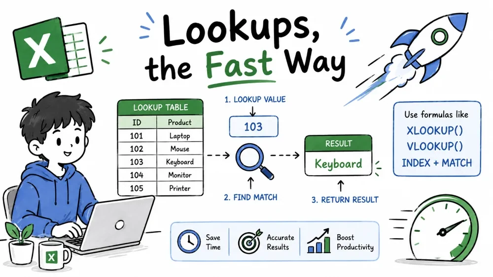
Lookups find a value in a table and pull back something related to it — the price for a product ID, the name behind an employee number. VLOOKUP and HLOOKUP are the classics, XLOOKUP is the modern replacement, and INDEX MATCH is the flexible option that works in every Excel version.

Table of Contents

• VLOOKUP
• HLOOKUP
• XLOOKUP
• INDEX MATCH
• Choosing the Right Lookup

VLOOKUP

VLOOKUP searches the first column of a table for a value and returns a cell from the same row, a set number of columns to the right. It's the classic "find the product, get its price" tool.

Syntax: =VLOOKUP(lookup_value, table_array, col_index_num, [range_lookup])

=VLOOKUP("A101", A2:D10, 3, FALSE)
=VLOOKUP(B2, Products!A2:D50, 4, FALSE)

The first line looks for "A101" in column A and returns whatever is 3 columns over — column C. The second looks up the ID in B2, searches the Products sheet, and returns the 4th column. FALSE at the end means "exact match only," which is what you want almost every time.

Common mistake: The value you search for must be in the first column of the table. VLOOKUP can never look to the left — if the ID is in column C, this function simply can't find it.

Note: TRUE (or leaving it blank) means approximate match — the closest value less than or equal to the lookup. It's only useful for sorted bands like tax tiers, and it silently returns wrong rows when you forget to sort.

HLOOKUP

HLOOKUP is the horizontal twin. It searches the first row for a value and returns a cell from the same column, a set number of rows down. Use it when your data is laid out in rows (periods across the top) rather than columns.

Syntax: =HLOOKUP(lookup_value, table_array, row_index_num, [range_lookup])

=HLOOKUP("Sales", A1:G4, 3, FALSE)

It finds "Sales" in the top row and returns the value 3 rows below it. Everything about VLOOKUP's FALSE and exact matching applies here too. In practice HLOOKUP is rare — most data is column-based — but it's worth recognizing when you see it in older workbooks.

XLOOKUP

XLOOKUP is the modern replacement for both VLOOKUP and HLOOKUP. It finds a value in one range and returns the matching value from another range — in any direction, left or right, with a built-in "not found" message. If you're on Excel 365, make this your default.

Syntax: =XLOOKUP(lookup_value, lookup_range, return_range, [if_not_found])

=XLOOKUP(B2, A2:A100, C2:C100)
=XLOOKUP(B2, A2:A100, C2:C100, "Not found")
=XLOOKUP(B2, A2:A100, B2:D100)

The lookup range and return range can be anywhere — nothing forces the ID to be in the first column anymore. The third line shows the real upgrade: return an entire row of results instead of a single cell.

Best practice: Always pass the if_not_found message. A blank lookup silently returns #N/A; a friendly "Not found" tells you (and anyone else) exactly what happened.

INDEX MATCH

INDEX returns the value at a specific row-and-column position in a range. MATCH finds the position of a value. Put them together and you get VLOOKUP's power with more freedom — and it works in every Excel version, not just 365.

Syntax: =INDEX(return_range, MATCH(lookup_value, lookup_range, 0))

=INDEX(C2:C100, MATCH("A101", A2:A100, 0))
=INDEX(B2:D50, MATCH(B2, A2:A50, 0), 3)

Read the first from the inside out: MATCH finds which row "A101" sits in, then INDEX returns that row's value from column C. The 0 means exact match. The second example uses MATCH for the row and 3 for the column directly, so INDEX pulls a specific cell — no range-swapping needed.

Note: Unlike VLOOKUP, INDEX MATCH looks left just as easily as right, and inserting a column in the middle of the table doesn't break it, because you reference the return range directly.

Choosing the Right Lookup

Ask AI to Write These Formulas (Copilot & ChatGPT)

Lookups have the most fiddly arguments of any formula family, so they're a perfect job for AI. Both Microsoft Copilot (in Excel 365) and ChatGPT can write them — just point at your table.

In Excel with Microsoft Copilot — open the Copilot chat pane and describe the match:

• "Use XLOOKUP to find the price for the product ID in B2 from the table in A2:D50."
• "Write a VLOOKUP that looks up the ID in A2 in the first column of Products and returns the 4th column, exact match."

With ChatGPT — give the ranges and ask for a specific function:

• "Write an INDEX MATCH formula that looks up the ID in A2 within A2:A100 and returns the matching value from C2:C100."
• "Which lookup should I use if the ID is to the right of the value I want to return? Give the formula."

Tip: Tell the AI exact match explicitly — "use FALSE / 0 for exact match." Otherwise it may hand you an approximate-match formula that quietly returns the wrong row.