Dynamic Arrays: FILTER, SORT & UNIQUE Done with a Single Spill

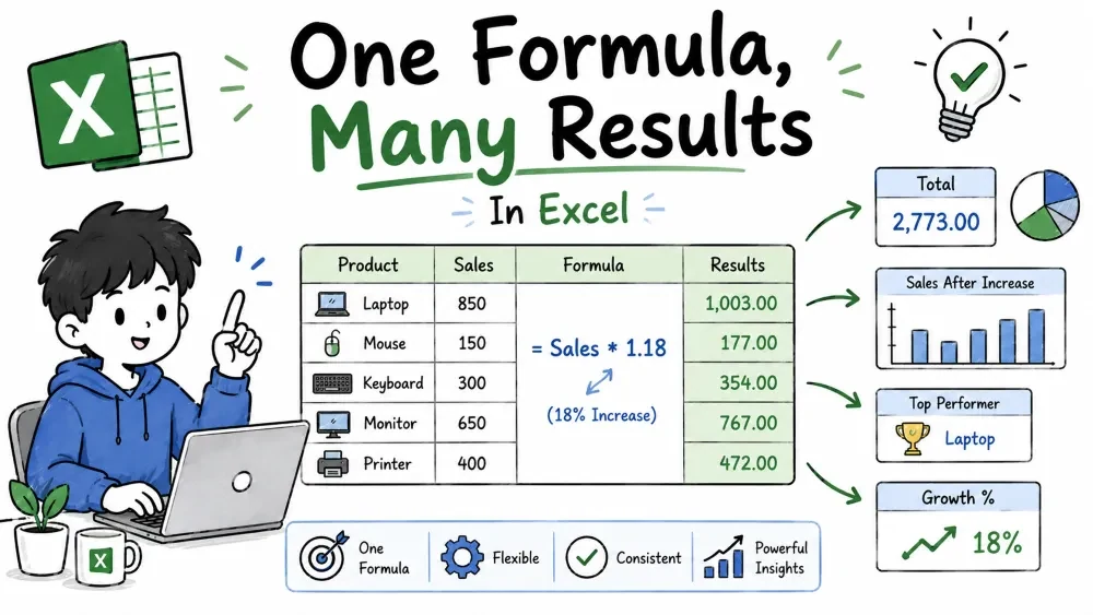
Dynamic arrays are Excel 365's biggest change in years: one formula now returns a whole range of results that spill into the cells beside it. FILTER selects the rows you want, SORT orders them, and UNIQUE strips out duplicates — no more dragging formulas down or rebuilding reports by hand.

Table of Contents

• What Are Dynamic Arrays?
• FILTER
• SORT
• UNIQUE
• Combining Dynamic Functions

What Are Dynamic Arrays?

In older Excel, a formula in one cell produced one result. With dynamic arrays, a formula can produce many results at once, and Excel "spills" them into the empty cells below or beside the formula automatically. You write the formula once in a single cell; the results fill themselves in.

=SORT(A2:A10)

Type that in B2 and the whole sorted list appears, each item dropping into the next row down. You never copy the formula into other cells. Anything you write that blocks the spill area triggers a #SPILL error — that's Excel telling you the results have nowhere to go.

FILTER

FILTER returns every row from a range that matches a condition. It's the dynamic replacement for the old "apply a filter and copy the visible rows" workflow.

Syntax: =FILTER(array, include, [if_empty])

=FILTER(A2:D20, B2:B20="West")
=FILTER(A2:D20, (B2:B20="West")*(C2:C20>100), "None")

The first line returns all rows where column B says "West". The include argument must be the same height as the array — that's how Excel knows which rows to keep. In the second example, * is the dynamic-array way of writing AND: a row only survives when both the region matches and the amount is over 100. The last argument gives a message when nothing matches.

SORT

SORT orders a range by one or more columns, up or down, without touching your original data.

Syntax: =SORT(array, [sort_index], [sort_order], [by_col])

=SORT(A2:C20, 2, 1)
=SORT(A2:C20, 3, -1)

The first sorts by column 2 in ascending order (1). The second sorts by column 3 descending (-1). The original data stays exactly as it was — the sorted copy appears wherever you typed the formula.

UNIQUE

UNIQUE returns the distinct values from a range — a one-formula de-duplication.

Syntax: =UNIQUE(array, [by_col], [exactly_once])

=UNIQUE(B2:B20)
=UNIQUE(B2:B20, FALSE, TRUE)

The first gives you every region/category that appears in the column, each once. The second shows the stricter mode: TRUE as the third argument returns only values that appear exactly once in the data — handy for spotting anomalies or orphaned records.

Combining Dynamic Functions

The real power is nesting them. You can filter first, then sort or dedupe the result, all in one formula. Each inner function hands its results straight to the outer one.

=SORT(FILTER(A2:C20, B2:B20="West"), 1, 1)
=UNIQUE(FILTER(B2:B20, C2:C20>100))

The first pulls the West rows, then sorts them by column 1 — one formula, both operations. The second filters to the high-value rows, then lists each unique region. Build from the inside out: decide what you want to keep (FILTER), then what you want done with it (SORT/UNIQUE).

Best practice: Build these step by step — get the FILTER working on its own first, then wrap it in SORT or UNIQUE. Debugging a nested formula is far easier when you've already confirmed the inner piece works.