TEXT Functions: Cleaning, Splitting & Reshaping Your Text

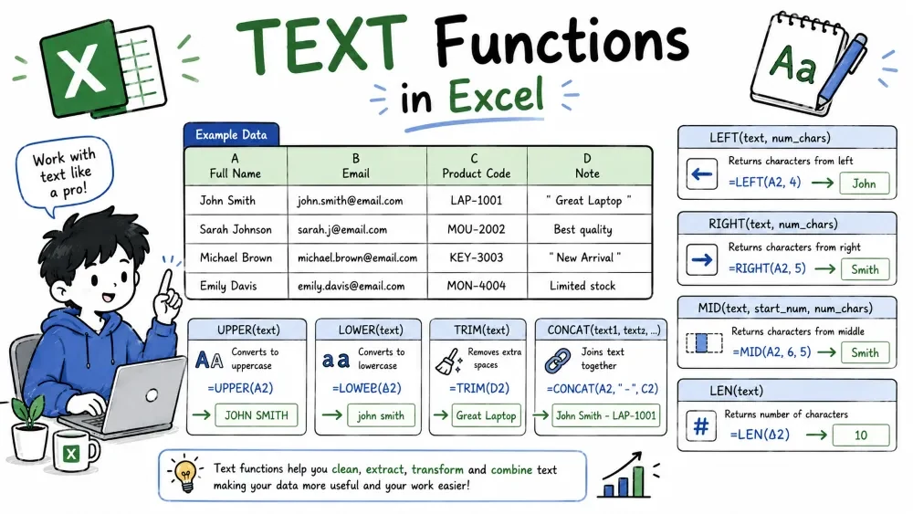
Text functions cut, clean, join, and reshape text. They're the tools of data cleaning — splitting full names, stripping stray spaces, standardizing case, and pulling IDs out of messy strings — so the rest of your formulas get clean input.

Table of Contents

• LEFT, RIGHT, MID
• LEN & TRIM
• CONCAT, CONCATENATE & TEXTJOIN
• UPPER, LOWER, PROPER
• SUBSTITUTE & REPLACE
• TEXT

LEFT, RIGHT, MID

These three pull characters out of a string. LEFT takes from the beginning, RIGHT from the end, and MID from anywhere in the middle.

Syntax: =LEFT(text, [num_chars]) — =RIGHT(text, [num_chars]) — =MID(text, start_num, num_chars)

=LEFT(A2, 3)
=RIGHT(A2, 4)
=MID(A2, 2, 5)

LEFT(A2, 3) returns the first 3 characters — an area code or a prefix. RIGHT(A2, 4) returns the last 4 — often a year or a code suffix. MID(A2, 2, 5) starts at character 2 and takes 5 characters from there. MID is the flexible one; LEFT and RIGHT are just its two special cases.

LEN & TRIM

LEN counts how many characters a cell contains. TRIM removes the extra spaces around and between words. They're the first thing you reach for when imported data looks wrong.

=LEN(A2)
=TRIM(A2)
=LEN(TRIM(A2))

LEN(A2) gives a character count — handy for spotting IDs of the wrong length. TRIM(A2) collapses " John Smith " into "John Smith", removing leading, trailing, and double spaces. LEN(TRIM(A2)) shows the true length after the spaces are gone.

Best practice: If lookups on text keep failing, suspect invisible spaces. TRIM them before comparing — a space at the end is the classic reason =VLOOKUP(...) suddenly returns #N/A.

CONCAT, CONCATENATE & TEXTJOIN

These join text together. CONCATENATE is the older name, CONCAT is its modern replacement, and TEXTJOIN adds a separator and can skip blank cells.

Syntax: =CONCATENATE(text1, [text2], ...) — =TEXTJOIN(delimiter, ignore_empty, text1, ...)

=CONCATENATE(A2, " ", B2)
=CONCAT(A2:B2)
=TEXTJOIN(" - ", TRUE, A2:C2)

The first builds a full name from first name (A2) and last name (B2) with a space between. CONCAT(A2:B2) joins a whole range at once. TEXTJOIN(" - ", TRUE, A2:C2) joins three cells separated by " - ", and TRUE tells it to skip any blanks — so a missing middle cell doesn't leave double separators.

UPPER, LOWER, PROPER

These standardize case. UPPER makes everything uppercase, LOWER makes it lowercase, and PROPER capitalizes the first letter of each word.

=UPPER(A2)
=LOWER(A2)
=PROPER(A2)

UPPER(A2) turns "john smith" into "JOHN SMITH". PROPER(A2) turns "john SMITH" into "John Smith" — the quick fix when a mailing list arrived with mixed caps.

SUBSTITUTE & REPLACE

Both swap part of a string, but they decide what to change differently. SUBSTITUTE replaces specific text wherever it appears; REPLACE replaces characters by position.

Syntax: =SUBSTITUTE(text, old_text, new_text, [instance_num]) — =REPLACE(old_text, start_num, num_chars, new_text)

=SUBSTITUTE(A2, "-", "")
=REPLACE(A2, 3, 2, "XX")

SUBSTITUTE(A2, "-", "") removes every dash — cleaning an ID like "AB-12-CD" into "AB12CD". REPLACE(A2, 3, 2, "XX") overwrites the two characters starting at position 3 with "XX", no matter what those characters are.

TEXT

TEXT changes how a number or date displays by converting it to text with a specific format. Use it when you need "1,234.50" or "05-Aug-2026" as a string, not just on screen.

Syntax: =TEXT(value, format_text)

=TEXT(A2, "0.00")
=TEXT(B2, "dd-mmm-yyyy")

TEXT(A2, "0.00") formats 1234.5 as "1234.50". TEXT(B2, "dd-mmm-yyyy") turns a date serial into "05-Aug-2026". The result is text, so you can concatenate it — but it's no longer a number, so you can't do math on it.