Advanced Pivot Tables — Calculated Fields, Data Models & Pro Refinements

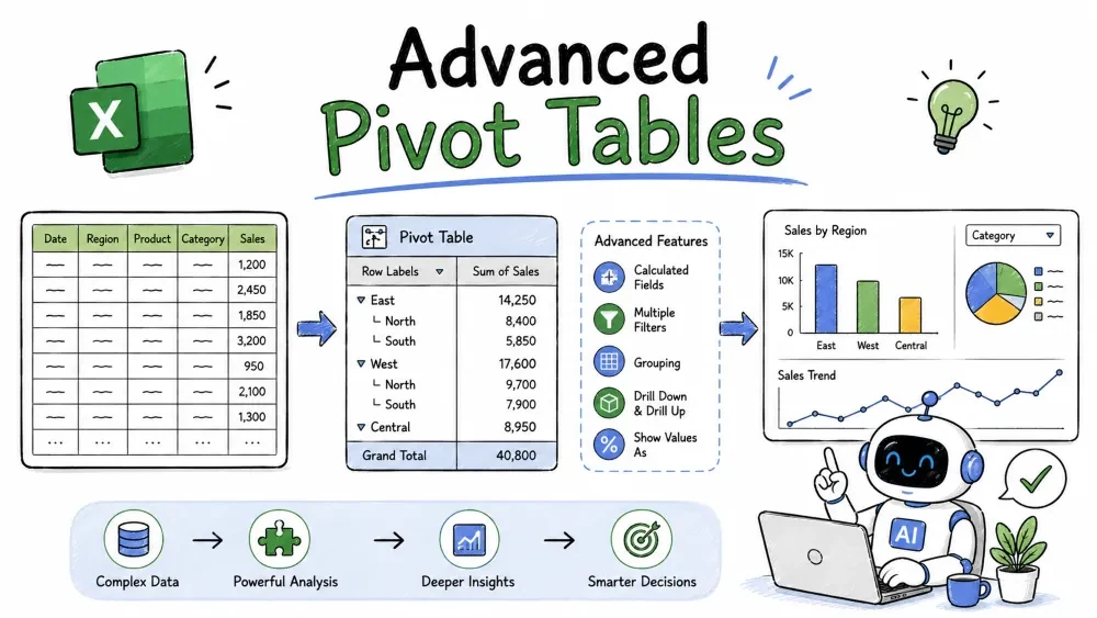
Once you can build and shape a pivot, the advanced techniques add real power: calculated fields, "show values as" calculations, smarter references with GETPIVOTDATA, combining multiple data sources, and styling.

Table of Contents

1. Calculated Fields
2. Calculated Items
3. Show Values As
4. GETPIVOTDATA References
5. Combine Multiple Data Sources
6. Consolidate Identical Sheets
7. Conditional Formatting on Pivots
8. Refresh & Change the Data Source
9. Do It with AI

Calculated Fields

A calculated field is a new value column computed from other columns in your source data — like Profit = Revenue − Cost.

1. Click inside the pivot.
2. PivotTable Analyze tab → Fields, Items & Sets → Calculated Field.
3. Name it Profit.
4. Build the formula = Revenue - Cost from the available fields.
5. Click Add, then OK.

Profit now appears in the Fields pane under Values, and its totals are shown like any other field.

Important: a calculated field does the math after summing. It computes SUM(Revenue) - SUM(Cost), not a per-row profit that gets summed. Keep that in mind when your formula divides or multiplies — the result is based on the totals, not individual rows.

Calculated Items

A calculated item adds a new category to a row or column field — a total like "Other" computed from existing items.

1. Put a field (like Product) in Rows.
2. Right-click any item → Fields, Items & Sets → Calculated Item.
3. In the formula box, add your items: = Widget - Gadget.
4. Click Add, then OK.

The new item appears in the list of that field. Unlike calculated fields, calculated items use the row-level values, so multiplying works on individual entries.

Note: calculated items only exist inside the pivot. They add a row to your summary but never touch the source sheet.

Show Values As

Right-click a value in the pivot → Show Values As offers ready-built calculations:

• % of Grand Total — each value as a share of the overall total.
• % of Column / Row Total — share within a single column or row.
• Running Total — cumulative sum down the field.
• Difference From — change against a previous period or item.

For example, switching Revenue to % of Grand Total immediately shows which region drives the biggest slice of sales.

GETPIVOTDATA References

When you type a formula that points at a pivot cell, Excel may insert a GETPIVOTDATA formula:

=GETPIVOTDATA("Revenue",$A$3,"Region","North")

That formula pulls one specific value (North's revenue) from the pivot. It's safe because it still works even if you move or reshape the pivot.

• If you'd rather write plain cell references, turn it off: PivotTable Analyze → Options → untick Generate GetPivotData.
• To use it better: type =, click a pivot cell, and Excel writes the formula for you.

Why it is useful: regular cell references break when the pivot grows or shrinks; GETPIVOTDATA follows the pivot wherever it goes.

Combine Multiple Data Sources

Modern Excel lets a pivot read from several tables at once via relationships:

1. When creating the pivot, tick Add this data to the Data Model.
2. Create a second, related table (for example a Product table with prices).
3. With the pivot selected, PivotTable Analyze → Relationships to link the two tables.
4. Fields from both tables now appear in one pivot.

This is Excel's answer to a small relational database — combine sales and product info without stacking them into one sheet.

Consolidate Identical Sheets

To merge several sheets with the same layout into one pivot:

1. Press Alt + D + P (the legacy PivotTable and PivotChart Wizard).
2. Choose Multiple consolidation ranges → Next.
3. Select Create a single page field for me.
4. Add each sheet's range, one at a time.
5. Click Finish.

All identical sheets roll into one pivot, with each source appearing in a page field you can toggle.

Tip for beginners using the classic wizard: the modern Insert → PivotTable dialog can't do this — this is the one case where you still need the old shortcut.

Conditional Formatting on Pivots

You can color cells based on their values, same as a normal range:

1. Select the numbers in the pivot.
2. Home → Conditional Formatting → Color Scales or Data Bars.
3. In the dialog, set the rule scope to All cells showing "Revenue" values so the format survives pivot changes.

Best practice: use the "All cells showing..." scope so the formatting follows the pivot around when you drag new fields in.

Refresh & Change the Data Source

• Refresh: right-click → Refresh, Data tab → Refresh All, or Ctrl + Alt + F5.
• Change source: PivotTable Analyze → Change Data Source → pick the new range. Useful when the data grows to a new block of rows.
• Turn the pivot back into plain data: copy the pivot cells → Paste Values to drop the summary into normal cells.

Do It with AI

This is where AI pulls the most weight — formulas.

• ChatGPT: prompt My Excel pivot has fields Revenue and Cost. Give me the Calculated Field formula for Profit and the exact menu path to add it. It returns = Revenue - Cost plus PivotTable Analyze → Fields, Items & Sets → Calculated Field.
• ChatGPT for GETPIVOTDATA: ask it to explain this formula and rewrite it for a different region — a fast way to learn how the reference works.
• Copilot in Excel: after adding the field, ask What is the total profit? to double-check the pivot's number against your own count.

Caution: AI can invent function names. Paste any generated formula into a cell and verify the result before it goes into a report.